
Bell's theorem
From Wikipedia, the free encyclopedia
Bell's theorem is the most famous legacy of the late physicist John S. Bell. It is famous for showing that the predictions of quantum mechanics (QM) are not intuitive, and touches upon fundamental philosophical issues that relate to modern physics. Bell's theorem states:
| “ | No physical theory of local hidden variables can ever reproduce all of the predictions of quantum mechanics. | ” |
Contents
|
[edit] Overview
As in the situation explored in the EPR paradox, Bell considered an experiment in which a source produces pairs of correlated particles. For example, a pair of particles with correlated spins is created; one particle is sent to Alice and the other to Bob. On each trial, each observer independently chooses between various detector settings and then performs an independent measurement on the particle. (Note: although the correlated property used here is the particles' spin, it could alternatively be any correlated "quantum state" that encodes exactly one quantum bit.)
| Same axis: | pair 1 | pair 2 | pair 3 | pair 4 | ...n | |
|---|---|---|---|---|---|---|
| Alice, 0°: | + | - | - | + | ... | |
| Bob, 180°: | + | - | - | + | ... | |
| Correlation: ( | +1 | +1 | +1 | +1 | ...)/n = +1 | |
| (100% identical) | ||||||
| Orthogonal axes: | pair 1 | pair 2 | pair 3 | pair 4 | ...n | |
| Alice, 0°: | + | - | + | - | ... | |
| Bob, 90°: | - | - | + | + | ... | |
| Correlation: ( | -1 | +1 | +1 | -1 | ...)/n = 0.0 | |
| (50% identical) |
When Alice and Bob measure the spin of the particles along the same axis (but in opposite directions), they get identical results 100% of the time. But when Bob measures at orthogonal (right) angles to Alice's measurements, they get identical results only 50% of the time. In terms of mathematics, the two measurements have a correlation of 1, or perfect correlation when read the same way; when read at right angles, they have a correlation of 0; no correlation. (A correlation of -1 would indicate getting opposite results for each measurement.)
So far, the results can be explained by positing local hidden variables — each pair of particles may have been sent out with instructions on how to behave when measured in the two axes (either '+' or '-' for each axis). Clearly, if the source only sends out particles whose instructions are identical for each axis, then when Alice and Bob measure on the same axis, they are bound to get identical results, either (+,+) or (-,-); but (if all four possible pairings of + and - instructions are generated equally) when they measure on perpendicular axes they will see zero correlation.
| Classical model: | spin | spin | spin | spin | spin | spin | spin | spin |
|---|---|---|---|---|---|---|---|---|
| Hidden variable for 0° (a): | + | + | + | + | - | - | - | - |
| Hidden variable for 45° (b): | + | + | + | - | - | - | - | + |
| Hidden variable for 90° (a'): | + | + | - | - | - | - | + | + |
| Hidden variable for 135° (b'): | + | - | - | - | - | + | + | + |
| Correlation: | ||||||||
| If measured on a-b, score: | +1 | +1 | +1 | -1 | +1 | +1 | +1 | -1 |
| If measured on a'-b, score: | +1 | +1 | -1 | +1 | +1 | +1 | -1 | +1 |
| If measured on a'-b', score: | +1 | -1 | +1 | +1 | +1 | -1 | +1 | +1 |
| If measured on a-b', score: | -1 | +1 | +1 | +1 | -1 | +1 | +1 | +1 |
| Expected average score: | +0.5 | +0.5 | +0.5 | +0.5 | +0.5 | +0.5 | +0.5 | +0.5 |
Now, consider that Alice or Bob can rotate their apparatus relative to each other by any amount at any time before measuring the particles, even after the particles leave the source. If local hidden variables determine the outcome of such measurements, they must encode at the time of leaving the source a result for every possible eventual direction of measurement, not just for the results in one particular axis.
Bob begins this experiment with his apparatus rotated by 45 degrees. We call Alice's axes a and a', and Bob's rotated axes b and b'. Alice and Bob then record the directions they measured the particles in, and the results they got. At the end, they will compare and tally up their results, scoring +1 for each time they got the same result and -1 for an opposite result - except that if Alice measured in a and Bob measured in b', they will score +1 for an opposite result and -1 for the same result.
Using that scoring system, any possible combination of hidden variables would produce an expected average score of at most +0.5. (For example, see table at the right, where the most correlated values of the hidden variables have an average correlation of +0.5, i.e. 75% identical. The unusual "scoring system" ensures that maximum average expected correlation is +0.5 for any possible system that relies on local hidden variables.)
| Randomized axes: | pair 1 | pair 2 | pair 3 | pair 4 | pair 5 | ...n | |
|---|---|---|---|---|---|---|---|
| Alice (axis, spin): | a', + | a', - | a, + | a', + | a, + | ... | |
| Bob (axis, spin): | b', + | b, - | b', - | b, - | b, + | ... | |
| Score: ( | +1 | +1 | +1 | -1 | +1 | ...)/n | =? |
Bell's Theorem shows that if the particles behave as predicted by quantum mechanics, Alice and Bob can score higher than the classical hidden variable prediction of +0.5 correlation; if the apparatuses are rotated at 45° to each other, quantum mechanics predicts that the expected average score is 0.71.
Quantum prediction in detail: When observations at an angle of θ are made on two entangled particles, the predicted correlation is cosθ. The correlation is equal to the length of the projection of the particle's vector onto his measurement vector; by trigonometry, cosθ. θ is 45°, and cosθ is
, for all pairs of axes except (a,b') – where they are 135° and
– but this last is taken in negative in the agreed scoring system, so the overall score is
Experiment reveals the 0.71 correlation predicted by quantum mechanics, so hidden variable theories cannot be correct (unless particles exchange information faster than light, which special relativity prohibits).
[edit] Importance of the theorem
This theorem has even been called "the most profound in science."[1] Bell's seminal 1964 paper was entitled "On the Einstein Podolsky Rosen paradox."[2] The Einstein Podolsky Rosen paradox (EPR paradox) assumes local realism, the intuitive notion that particle attributes have definite values independent of the act of observation and that physical effects have a finite propagation speed. Bell showed that local realism leads to a requirement for certain types of phenomena that are not present in quantum mechanics. This requirement is called Bell's inequality.
After EPR (Einstein-Podolsky-Rosen), quantum mechanics was left in an unsatisfactory position: either it was incomplete, in the sense that it failed to account for some elements of physical reality, or it violated the principle of finite propagation speed of physical effects. In a modified version of the EPR thought experiment, two observers, now commonly referred to as Alice and Bob, perform independent measurements of spin on a pair of electrons, prepared at a source in a special state called a spin singlet state. It was a conclusion of EPR that once Alice measured spin in one direction (e.g. on the x axis), Bob's measurement in that direction was determined with certainty, whereas immediately before Alice's measurement, Bob's outcome was only statistically determined. Thus, either the spin in each direction is not an element of physical reality, or the effects travel from Alice to Bob instantly.
In QM, predictions were formulated in terms of probabilities — for example, the probability that an electron might be detected in a particular region of space, or the probability that it would have spin up or down. The idea persisted, however, that the electron in fact has a definite position and spin, and that QM's weakness was its inability to predict those values precisely. The possibility remained that some yet unknown, but more powerful theory, such as a hidden variables theory, might be able to predict those quantities exactly, while at the same time also being in complete agreement with the probabilistic answers given by QM. If a hidden variables theory were correct, the hidden variables were not described by QM, and thus QM would be an incomplete theory.
The desire for a local realist theory was based on two assumptions:
- Objects have a definite state that determines the values of all other measurable properties, such as position and momentum.
- Effects of local actions, such as measurements, cannot travel faster than the speed of light (as a result of special relativity). If the observers are sufficiently far apart, a measurement taken by one has no effect on the measurement taken by the other.
In the formalization of local realism used by Bell, the predictions of theory result from the application of classical probability theory to an underlying parameter space. By a simple (but clever) argument based on classical probability, he then showed that correlations between measurements are bounded in a way that is violated by QM.
Bell's theorem seemed to put an end to local realist hopes for QM. Per Bell's theorem, either quantum mechanics or local realism is wrong. Experiments were needed to determine which is correct, but it took many years and many improvements in technology to perform them.
Bell test experiments to date overwhelmingly show that the inequalities of Bell's theorem are violated. This provides empirical evidence against local realism. They are also taken as positive evidence in favor of QM. The principle of special relativity is saved by the no-communication theorem, which proves that the observers cannot use the inequality violations to communicate information to each other faster than the speed of light.
John Bell's papers examined both John von Neumann's 1932 proof of the incompatibility of hidden variables with QM and Albert Einstein and his colleagues' seminal 1935 paper on the subject.
[edit] Slippery quantum properties
The following example[3] illustrates and makes the nature of Bell inequalities easy to understand. Consider a particle with a slippery shape property that is either square or round, depending on which way we look at it. The particle cannot be seen from two directions at once, and looking at it changes how it might have looked from other directions. A source creates entangled pairs of these particles, so that if we look at the two from the same angle they have the same shape, and sends them in opposite directions. Shape detectors independent of each other and of the source are placed in the path of each particle and randomly change between three observing angles after the particles are emitted. Because the particles are entangled, the detectors report the same shape every time they happen to measure a pair from the same observation angle. Additionally the detectors measure the same shape for half of all runs when they are set arbitrarily and independently to one of the three angles. This last property does hold for some real systems, and is the key Bell found to show the existence of alocality.
To construct a local model for this situation, we must assume that the information for shape appearance at each angle is carried on the particles. This is the only local way to ensure that the same shape is measured every time the detector angles happen to be the same. We can represent this information by either an s (for square) or r (for round) in each of three slots corresponding to the three detector angles. Remember that we can only observe the shape from one angle at a time, and subsequent measurement will not reflect what the shape would have been if we had observed it from another angle. Thus we can learn only two of the three pieces of information by measurement, one from each particle. The unobserved value in each particle's instruction set is an unknowable, hidden variable. Suppose a pair of entangled particles which would look square from angles 1 and 2 and round from angle 3 each carry the instruction set ssr. For this particular instruction set, there are five possible detector settings which yield the same shape (11,22,33,12,21) and four settings which yield different shapes (13,23,32,31), so with random detector settings, the probability of detecting the same shape given this instruction set is  . There are five more possible instruction sets (rss,srs,rrs,rsr,srr) that also give probability for detecting the same shape. The only other possible instruction sets in this local model are rrr and sss, for which the same shape is measured with probability 1. Whatever the distribution of these instruction sets among the entangled pairs, the detectors will measure the same shape in at least of all runs.
The Bell inequalities predict this for any local hidden variable model:
 ,
,
where Plhv is the proportion over all runs that a classical local hidden variables model predicts the detectors to measure the same shape. However, quantum mechanics predicts, and actual observation reveals, that the same shape appears in only half of all runs. Our inequality is violated:
 ,
,
where Pqm is the proportion over all runs that quantum mechanics predicts (and actual observation reveals) the detectors to measure the same shape. So, local hidden variable models do not adequately describe the system.
Note: Such a system can be created physically with spin-entangled electron/positron pairs substituted for the shape-entangled particles, and Stern-Gerlach analyzers substituted for shape detectors. The angles 0°, 120° and 240° give P = 1/2. Alternatively, the analog for a polarization entangled photon system is polarization detectors at angles 0°, 60° and 120° but because the linear polarizers only pass the vertical polarization of its rotated basis, measurements must be taken at the orthogonal angles as well.
[edit] Bell Inequalities
Bell inequalities concern measurements made by observers on entangled pairs of particles that have interacted and then separated. Hidden variable assumptions assume local realism, limiting the correlation of subsequent measurements of the particles. Different authors subsequently derived similar inequalities, collectively termed Bell inequalities. The inequalities assume that each quantum-level object has a well defined state that accounts for all its measurable properties and that distant objects do not exchange information faster than the speed of light. These well defined properties are often called hidden variables, the properties that Einstein posited when he stated his famous objection to quantum mechanics: "God does not play dice."
Bell showed that under quantum mechanics, which lacks local hidden variables, the inequalities (the correlation limit) may be violated. Instead, properties of a particle are not clear to verify in quantum mechanics but may be correlated with those of another particle due to quantum entanglement, allowing their state to be well defined only after a measurement is made on either particle. That restriction agrees with the Heisenberg uncertainty principle, a fundamental concept in quantum mechanics.
In Bell's work:
| “ | Theoretical physicists live in a classical world, looking out into a quantum-mechanical world. The latter we describe only subjectively, in terms of procedures and results in our classical domain. (...) Now nobody knows just where the boundary between the classical and the quantum domain is situated. (...) More plausible to me is that we will find that there is no boundary. The wave functions would prove to be a provisional or incomplete description of the quantum-mechanical part. It is this possibility, of a homogeneous account of the world, which is for me the chief motivation of the study of the so-called "hidden variable" possibility. (...) A second motivation is connected with the statistical character of quantum-mechanical predictions. Once the incompleteness of the wave function description is suspected, it can be conjectured that random statistical fluctuations are determined by the extra "hidden" variables -- "hidden" because at this stage we can only conjecture their existence and certainly cannot control them. (...) A third motivation is in the peculiar character of some quantum-mechanical predictions, which seem almost to cry out for a hidden variable interpretation. This is the famous argument of Einstein, Podolsky and Rosen. (...) We will find, in fact, that no local deterministic hidden-variable theory can reproduce all the experimental predictions of quantum mechanics. This opens the possibility of bringing the question into the experimental domain, by trying to approximate as well as possible the idealized situations in which local hidden variables and quantum mechanics cannot agree | ” |
In probability theory, repeated measurements of system properties can be regarded as repeated sampling of random variables. In Bell's experiment, Alice can choose a detector setting to measure either A(a) or A(a') and Bob can choose a detector setting to measure either B(b) or B(b'). Measurements of Alice and Bob may be somehow correlated with each other, but the Bell inequalities say that if the correlation stems from local random variables, there is a limit to the amount of correlation one might expect to see.
In addition to Bell's original inequality,[2] the form given by John Clauser, Michael Horne, Abner Shimony and R. A. Holt,[4] (the CHSH form) is especially important[4], as it gives classical limits to the expected correlation for the above experiment conducted by Alice and Bob:
![\ (1) \quad \mathbf{C}[A(a), B(b)] + \mathbf{C}[A(a), B(b')] + \mathbf{C}[A(a'), B(b)] - \mathbf{C}[A(a'), B(b')]\leq 2,](http://upload.wikimedia.org/math/8/b/e/8bea765f4463fcc1702ce8d6fd556689.png)
where C denotes correlation.
Correlation of observables X, Y is defined as

This is non-normalized form of the correlation coefficient considered in statistics (see Quantum correlation).
In order to formulate Bell's theorem, we formalize local realism as follows:
- There is a probability space Λ and the observed outcomes by both Alice and Bob result by random sampling of the parameter
 .
. - The values observed by Alice or Bob are functions of the local detector settings and the hidden parameter only. Thus
-
-
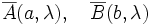
- Value observed by Alice with detector setting a is A(a,λ)
- Value observed by Bob with detector setting b is B(b,λ)
-
Implicit in assumption 1) above, the hidden parameter space Λ has a probability measure ρ and the expectation of a random variable X on Λ with respect to ρ is written
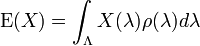
where for accessibility of notation we assume that the probability measure has a density.
Bell's inequality. The CHSH inequality (1) holds under the hidden variables assumptions above.
For simplicity, let us first assume the observed values are +1 or −1; we remove this assumption in Remark 1 below.
Let . Then at least one of

is 0. Thus


and therefore


Remark 1. The correlation inequality (1) still holds if the variables A(a,λ), B(b,λ) are allowed to take on any real values between -1, +1. Indeed, the relevant idea is that each summand in the above average is bounded above by 2. This is easily seen to be true in the more general case:


To justify the upper bound 2 asserted in the last inequality, without loss of generality, we can assume that
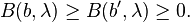
In that case

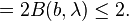 .
.
Remark 2. Though the important component of the hidden parameter λ in Bell's original proof is associated with the source and is shared by Alice and Bob, there may be others that are associated with the separate detectors, these others being independent. This argument was used by Bell in 1971, and again by Clauser and Horne in 1974,[5] to justify a generalisation of the theorem forced on them by the real experiments, in which detector were never 100% efficient. The derivations were given in terms of the averages of the outcomes over the local detector variables. The formalisation of local realism was thus effectively changed, replacing A and B by averages and retaining the symbol λ but with a slightly different meaning. It was henceforth restricted (in most theoretical work) to mean only those components that were associated with the source.
However, with the extension proved in Remark 1, CHSH inequality still holds even if the instruments themselves contain hidden variables. In that case, averaging over the instrument hidden variables gives new variables:
on Λ which still have values in the range [-1, +1] to which we can apply the previous result.
[edit] Original Bell's inequality
The original inequality that Bell derived was:[2]
 ,
,
where C is the "correlation" of the particle pairs and a, b and c settings of the apparatus. This inequality is not used in practice. For one thing, it is true only for genuinely "two-outcome" systems, not for the "three-outcome" ones (with possible outcomes of zero as well as +1 and −1) encountered in real experiments. For another, it applies only to a very restricted set of hidden variable theories, namely those for which the outcomes on both sides of the experiment are always exactly anticorrelated when the analysers are parallel, in agreement with the quantum mechanical prediction.
[edit] Bell's theorem: Bell inequalities are violated by some quantum predictions
Bell's theorem shows that quantum mechanics makes predictions that violate a "Bell inequality" in the setup considered in the EPR thought experiment.
In the usual quantum mechanical formalism, observables X, Y are represented as self-adjoint operators on a Hilbert space. To compute the correlation, assume that X, Y are represented by matrices in a finite dimensional space and that X, Y commute; this special case suffices for our purposes below. We then use the von Neumann measurement postulate: a series of measurements of an observable X on a series of identical systems in state φ produces a distribution of real values. By the assumption that observables are finite matrices, this distribution is discrete. The probability of observing λ is non-zero if and only if λ is an eigenvalue of the matrix X and moreover the probability is

where EX (λ) is the projector corresponding to the eigenvalue λ. The system state immediately after the measurement is

From this, we can show that the correlation of commuting observables X, Y in a pure state ψ is

We apply this fact in the context of the EPR paradox. The measurements performed by Alice and Bob are spin measurements for an electron. Alice can choose between two detector settings labelled a and a′; these settings correspond to measurement of spin along the z or the x axis. Bob can choose between two detector settings labelled b and b′; these correspond to measurement of spin along the z′ or x′ axis, where the x′ – z′ coordinate system is rotated 45° relative to the x – z coordinate system. The spin observables are represented by the 2 × 2 self-adjoint matrices:


These are the Pauli spin matrices normalized so that the corresponding eigenvalues are +1, −1. As is customary, we denote the eigenvectors of Sx by
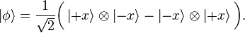
Let φ be the spin singlet state for a pair of electrons discussed in the EPR paradox. This is a specially constructed state described by the following vector in the tensor product
Now let us apply the CHSH formalism to the measurements that can be performed by Alice and Bob.


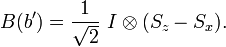
The operators B(b'), B(b) correspond to Bob's spin measurements along x′ and z′. Note that the A operators commute with the B operators, so we can apply our calculation for the correlation. In this case, we can show that the CHSH inequality fails. In fact, a straightforward calculation shows that

and
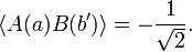
so that

Bell's Theorem: If the quantum mechanical formalism is correct, then the system consisting of a pair of entangled electrons cannot satisfy the principle of local realism. Note that  is indeed the upper bound for quantum mechanics, it's called Tsirelson's bound. The operators giving this maximal value are always isomorphic to the Pauli matrices.
[edit] Bell test experiments
Experimental tests can determine whether the Bell inequalities required by local realism hold up to the empirical evidence.
Bell's inequalities are tested by "coincidence counts" from a Bell test experiment such as the optical one shown in the diagram. Pairs of particles are emitted as a result of a quantum process, analysed with respect to some key property such as polarisation direction, then detected. The setting (orientations) of the analysers are selected by the experimenter.
Bell test experiments to date overwhelmingly suggest that Bell's inequality is violated. Indeed, a table of Bell test experiments performed prior to 1986 is given in 4.5 of Redhead, 1987.[6] Of the thirteen experiments listed, only two reached results contradictory to quantum mechanics; moreover, according to the same source, when the experiments were repeated, "the discrepancies with QM could not be reproduced".
The source S produces pairs of "photons", sent in opposite directions. Each photon encounters a two-channel polariser whose orientation (a or b) can be set by the experimenter. Emerging signals from each channel are detected and coincidences of four types (++, --, +- and -+) counted by the coincidence monitor.
Nevertheless, the issue is not conclusively settled. According to Shimony's 2004 Stanford Encyclopedia overview article[7]
- "Most of the dozens of experiments performed so far have favored Quantum Mechanics, but not decisively because of the 'detection loopholes' or the 'communication loophole.' The latter has been nearly decisively blocked by a recent experiment and there is a good prospect for blocking the former."
To explore the 'detection loophole', one must distinguish the classes of homogeneous and inhomogeneous Bell inequality.
[edit] Two classes of Bell inequality
The standard assumption in Quantum Optics is that "all photons of given frequency, direction and polarization are identical" so that photodetectors treat all incident photons on an equal basis. Such a fair sampling assumption generally goes unacknowledged, yet it effectively limits the range of local theories to those which conceive of the light field as corpuscular. The assumption excludes a large family of local realist theories, in particular, Max Planck's description. We must remember the cautionary words of Albert Einstein[8] shortly before he died: "Nowadays every Tom, Dick and Harry ('jeder Kerl' in German original) thinks he knows what a photon is, but he is mistaken".
Objective physical properties for Bell’s analysis (local realist theories) include the wave amplitude of a light signal. Those who maintain the concept of duality, or simply of light being a wave, recognize the possibility or actuality that the emitted atomic light signals have a range of amplitudes and, furthermore, that the amplitudes are modified when the signal passes through analyzing devices such as polarizers and beam splitters. It follows that not all signals have the same detection probability (Marshall and Santos 2002[1]).
The fair sampling problem was faced openly in the 1970s. In early designs of their 1973 experiment, Freedman and Clauser[9] used fair sampling in the form of the Clauser-Horne-Shimony-Holt (CHSH[4]) hypothesis. However, shortly afterwards Clauser and Horne[5] made the important distinction between inhomogeneous (IBI) and homogeneous (HBI) Bell inequalities. Testing an IBI requires that we compare certain coincidence rates in two separated detectors with the singles rates of the two detectors. Nobody needed to perform the experiment, because singles rates with all detectors in the 1970s were at least ten times all the coincidence rates. So, taking into account this low detector efficiency, the QM prediction actually satisfied the IBI. To arrive at an experimental design in which the QM prediction violates IBI we require detectors whose efficiency exceeds 82% for singlet states, but have very low dark rate and short dead and resolving times. This is well above the 30% achievable (Brida et al. 2006[2]) so Shimony’s optimism in the Stanford Encyclopedia, quoted in the preceding section, appears over-stated.
[edit] "Loophole" or new phenomenon?
Clauser and Horne[5] recognized that, because of the limitations of light detectors, an experimental test between quantum optics and local realist theories was possible only with some restriction on the range of local theories to be considered. They introduced the No Enhancement Hypothesis (NEH):
a light signal, originating in an atomic cascade for example, has a certain probability of activating a detector. Then, if a polarizer is interposed between the cascade and the detector, the detection probability cannot increase.
Given NEH, we may derive an HBI between coincidence rates with polarizers in place and coincidence rates without one or both polarizers.
This was made the basis of the experiment of Freedman and Clauser[9], in which the HBI was found to be violated. That implies NEH plus locality cannot be true. As locality (or, what is the same thing, causality) is basic to science, it follows that NEH is not true. Thus the Freedman-Clauser experiment reveals the reality of a new phenomenon, namely, signal enhancement. Let us be explicit.
In the total set of signals from an atomic cascade there is a subset whose detection probability increases as a result of passing through a linear polarizer.
This is perhaps not surprising, as it is known that adding noise to data can, in the presence of a threshold, help reveal hidden signals (this property is known as stochastic resonance[3]). One cannot conclude that this is the only local-realist alternative to Quantum Optics, but it does show that the word loophole is ideologically loaded. Moreover, the analysis leads us to recognize that the Bell-inequality experiments, far from showing a breakdown of realism or locality, are capable of revealing important new phenomena.
[edit] Implications of violation of Bell's inequality
The phenomenon of quantum entanglement that is behind violation of Bell's inequality is just one element of quantum physics which cannot be represented by any classical picture of physics; other non-classical elements are complementarity and wavefunction collapse. The problem of interpretation of quantum mechanics is intended to provide a satisfactory picture of these non-classical elements of quantum physics.
Some advocates of the hidden variables idea believe that experiments have ruled out local hidden variables. They are ready to give up locality, explaining the violation of Bell's inequality by means of a "non-local" hidden variable theory, in which the particles exchange information about their states. This is the basis of the Bohm interpretation of quantum mechanics. It is however, requiring for example, that all particles in the universe be able to instantaneously exchange information with all others.
Finally, one subtle assumption of the Bell inequalities is counterfactual definiteness. The derivation refers to several objective properties that cannot all be measured for any given particle, since the act of taking the measurement changes the state. Under local realism the difficulty is readily overcome, so long as we can assume that the source is stable, producing the same statistical distribution of states for all the subexperiments. If this assumption is felt to be unjustifiable, though, one can argue that Bell's inequality is unproven. In the Everett many-worlds interpretation, the assumption of counterfactual definiteness is abandoned, this interpretation assuming that the universe branches into many different observers, each of whom measures a different observation. Hence many worlds can adhere to both the properties of philosophical realism and the principle of locality and not violate Bell's conditions.
[edit] Notable quotations
Heinz Pagels, in The Cosmic Code, writes:
| “ | Some recent popularizers of Bell's work when confronted with [Bell's inequality] have gone on to claim that telepathy is verified or the mystical notion that all parts of the universe are instantaneously interconnected is vindicated. Others assert that this implies communication faster than the speed of light. That is rubbish; the quantum theory and Bell's inequality imply nothing of this kind. Individuals who make such claims have substituted a wish-fulfilling fantasy for understanding. If we closely examine Bell's experiment we will see a bit of sleight of hand by the God that plays dice which rules out actual nonlocal influences. Just as we think we have captured a really weird beast--like acausal influences--it slips out of our grasp. The slippery property of quantum reality is again manifested. | ” |